For years, people smarter than me have been telling me to get into Python. I’ve had a perfectly valid reason to resist. It seemed difficult. And besides, just look at the syntax! It looks like some silly BASIC that I used to code back in the 1980’s. It doesn’t even have any semi colons! But slowly I’m starting to see the light. There actually seem to be some hidden logic to the madness.
Now there’s an important point to remember while reading this and upcoming articles on the subject of Python. You are reading an article by someone who is just learning about the topic. You’re not reading an instruction manual by an expert. That’s right. These are the ramblings of someone who probably know less than you do on the topic.
Keep that in mind when commenting on the article below. Do you think that I’m wrong about something? You know a better way? You’re probably right. Feel free to make your suggestions below.
In the past week or so, I’ve read a couple of books on Python. Well, I’ve read part of them anyhow. As good as these books seem, they’re also a reminder for me about my own preferred way of learning. Hands on.
Those of you out there who are unlucky enough to have had to study a grammatically complex language like Latin or German, know that linguists, no matter how cunning they are, tend to over complicate. They fall in love with the grammar. Instead of teaching you how to start communicating in German, they’ll spend years making you memorize terminology and rules around dative, accusative, nominative and how implied movement causes words to change and your grades to fall. Well, I prefer to start trying to speak it and the grammar will have to wait.
So for that reason, in this first article, we’re going to learn by doing. We’re going to use a ready-to-use Python environment. We’re not going to pip anything and we’re not going to mention words like tuple. Well, not anymore.
If you, like me, are used to C# or something similar, then it is quite jarring to enter the Python world. The first question from a C# point of view would be to ask for which software to develop in. That’s quite a complex topic actually, so let’s skip that for this article. For now, we’re going to use Quantopian.
Quantopian is a web based development environment for trading simulations. It’s totally free and easy to get started with. You can do fairly much in that environment, but as a web environment it obviously has some limitations. Depending on who you are and what you aim to do, Quantopian may be sufficient for your needs, or it may be severely limiting. Either way, it’s a good place to start.
A nice thing about Quantopian, apart from that they are free, is that they are swimming in VC cash. They’re spending money on their platform and they have a large development team. It’s not a little garage operation anymore. Well, technically, Quantopian started in a garden shed and not a garage… If you work on their web platform, you’ll get full access to minute level data for stocks, fundamental data and a whole bunch of things that would otherwise cost you a lot.
So what’s in it for them? Well, their plan is to create a hedge fund based on the best of what people can make on their platform, and pay a cut to those who contribute. Will that work? Perhaps. Who knows. Let’s see. I like the guys behind Quantopian (hi Fawce!) and I hope they pull it off. If you are good at quant modeling, this may be a good chance to get into the business.
At the moment, Quantopian only supports US stocks. As a beta tester, I have tried their upcoming futures data as well. A few bugs aside, it looks like a solid implementation. In our first example, we’ll just make an equity model though.
Let’s design a simple equity momentum model to learn by example. It’s not meant to be The Model to Rule All Models. This is just an average momentum model. One you can easily improve upon yourself.
Our rules:
- Investment Universe: Top 500 US stocks by market cap.
- Trading frequency: Monthly
- Stock selection: Top momentum stocks at start of each month.
- Momentum analytic: 90 day regression slope multiplied by R2.
- Minimum momentum to be accepted: 30
- Number of stocks in portfolio: 30
- Position weights: 1/30 (equal weighted)
Quantopian does not, unfortunately, have actual S&P membership data yet. They do however have historical market cap data. They even made a useful function for us to automagically get the top 500 stocks by market cap dynamically. So let’s use that as a proxy for the index.
The rules above are quite simple. Still, if you were to write this model in C# using RightEdge, it would require quite a bit of code. The first thing I realized when tinkering with Python is just how little code is actually needed. That means that you can build things very quickly. It also means that it becomes so much easier to read the code. Which of course, is the entire point here.
Ok, so let’s construct this sucker.
If you haven’t already, head over to Quantopian and make an account. Then create a new algorithm. It’s just there in the menus. Go on, make a new one.
When you make a new algorithm, you’ll get some template code. You can tinker with this later. For now, just delete it.
First, we need to add a few import statements. These are just like Using statements in C#. We just need to tell the code which libraries we want to use. From the standard template, all I’ve added are those two at the bottom, numpy and scipy. These are libraries you will want to dig into later, as they are very useful. For now, just know that numpy is great for playing with math and scipy has some neat statistics functions that we need.
|
1 2 3 4 5 6 7 8 9 10 11 |
""" This is a simple demo model using equity momentum. """ from quantopian.algorithm import attach_pipeline, pipeline_output from quantopian.pipeline import Pipeline from quantopian.pipeline.data.builtin import USEquityPricing from quantopian.pipeline.factors import AverageDollarVolume from quantopian.pipeline.filters.morningstar import Q500US import numpy as np from scipy import stats |
In the rules we defined, there’s only really one even remotely tricky thing. The momentum calculation. But don’t worry. No need for making a new class, defining an indicator, iterating series and doing step by step calculations. Here’s the function for the annualized standard deviation, adjusted for R2:
|
1 2 3 4 5 |
def _slope(ts): x = np.arange(len(ts)) slope, intercept, r_value, p_value, std_err = stats.linregress(x, ts) annualized_slope = (np.power(np.exp(slope), 250) -1) *100 return annualized_slope * (r_value ** 2) |
Let’s stop and take a look at this function. It really illustrates the Python beauty. It also differs starkly from how things would be done in C#.
The input to this function is a time series. Actually, a whole bunch of them. We’re just going to throw a huge amount of log data at this function, and it will respond with the value we’re looking for. So expected incoming value here is a log series.
The first line creates our x series. Function arange will return a series of [1, 2, 3, 4, …] with as many points as our series. Neat, huh?
Then we calculate the various statistics associated with linear regression on the second row. The linregress function outputs five different values. We only need two of them. Keep in mind again that the incoming ts is already logs, so it’s perfectly fine to apply the linear regression on it.
Next step is to get the annualized slope. Now the expression exp(slope) would give us the daily percentage slope, if you remember your Statistics 101 class. If for instance the slope value is 1.01 that means that the regression line over the measured period moved up by 1% per day. To annualize it, we’ll need to raise it to the power of 250 and remove 1. Then let’s just multiply by 100 to make it easier to read.
Fine, let’s move on. The rest is simpler. Next we’ll set the necessary things in the startup section. A function called initialize will be run automatically when you execute.
|
1 2 3 4 5 6 7 8 9 10 11 12 13 14 15 |
def initialize(context): """ Called once at the start of the algorithm. """ # Setting global parameters context.momentum_window = 90 context.minimum_momentum = 30 context.number_of_stocks = 30 # -------------------------- # Rebalance monthly schedule_function(my_rebalance, date_rules.month_start(), time_rules.market_open(hours=1)) # Create our dynamic stock selector. attach_pipeline(make_pipeline(), 'us_500') |
We do three things here. At the top, you see some settings. The context object is where we set global things. Stuff we want to reference later in other places. So let’s use this for a few input settings for our model, such as the time window and number of stocks.
Experienced programmers from C type languages surely ask how we can just make stuff up like this. Well, in Python there’s no need to declare variables or even typecast them. If you write x=5 you suddenly have a new variable called x of type integer. It’s all automatic. In the case of the context object, it’s kinda a special case, so just go with it. This object is made to be extended in this manner, and we can tag any type of data we want to it, with any name we want.
The rebalance function is quite neat. In my own C# momentum models, my logic for determining rebalance day has more lines the entire Python model. Here, we just set a scheduler. Using built in stuff, we just write one line that tells the code to run function my_rebalance on the first day of the month. Done.
Lastly, we need to create our pipeline. This is a somewhat unfortunate name, in that it doesn’t exactly add clarity. What we’re doing here is to create an object which is going to help us fetch a list of the top 500 stocks any time we ask for it.
That function, the one that gets the top 500 stocks, is shown below. Don’t worry about it for now. You can simply copy it and use as is.
|
1 2 3 4 5 6 7 8 9 10 11 12 13 14 15 |
def make_pipeline(): """ This will return the top 500 US stocks by market cap, dynically updated. """ # Base universe set to the Q500US base_universe = Q500US() yesterday_close = USEquityPricing.close.latest pipe = Pipeline( screen = base_universe, columns = { 'close': yesterday_close, } ) return pipe |
Well then. Ready to move on to the final part of the model? The actual trading.
The function my_rebalance will be executed at the start of each month, as we set before in the schedule function. This is where the magic happens. Here’s what we need to do at rebalance time:
- Update the investment universe, so it only includes the current top 500 stocks.
- Create a ranking list. Sort it, and select top 30 stocks.
- Sell any stock that’s not in the ranking list.
- Check the buy list to make sure the momentum slope is higher than our limit (30).
- Calculate the weight. We’re using equal weight, so a simple 1/30 will do.
- Trade!
If you think that the code below are shockingly few lines to do all of this, keep in mind that I have deliberately used more lines than necessary to make it easier to follow. It can be done much shorter.
|
1 2 3 4 5 6 7 8 9 10 11 12 13 14 15 16 17 18 19 20 21 22 23 24 25 |
def my_rebalance(context,data): """ Our monthly rebalancing """ context.output = pipeline_output('us_500') # update the current top 500 us stocks context.security_list = context.output.index momentum_list = np.log(data.history(context.security_list, "close", context.momentum_window, "1d")).apply(_slope) ranking_table = momentum_list.sort_values(ascending=False) # Sorted buy_list = ranking_table[:context.number_of_stocks] # These we want to buy # Let's trade! for security in context.portfolio.positions: if security not in buy_list: order_target(security, 0) # If a stock in the portfolio is not in buy list, sell it! for security in context.security_list: if security in buy_list: if buy_list[security] < context.minimum_momentum: weight = 0.0 else: weight = 1.0 / context.number_of_stocks # Equal size to keep simple order_target_percent(security, weight) # Trade! |
The first two lines just update our list of securities. We only want to trade stocks that were part of the top 500 largest stocks by market cap at the time, and this function takes care of that for us.
The third line is the most interesting thing in the entire code. At least in my view. Here we do something which would require quite a bit of code in most other environments. And we do it in one line.
Stop for a moment and look at this line. Let’s break it down.
|
1 |
momentum_list = np.log(data.history(context.security_list, "close", context.momentum_window, "1d")).apply(_slope) |
The part data.history(context.security_list, “close”, context.momentum_window, “1d”) gets our time series data. This essentially means “Get me time series data for all 500 stocks in the investment universe, for the past 90 days, using daily frequency”. Yes, it does all of that.
Then there is the function np.log, which will turn the entire thing into log series. All of it. the 500 prices series. Finally, we apply our first function, _slope, on the whole thing. Take that C#!
Here we just fetched 90 data points for 500 stocks, turned them into logs, threw them at a function that makes adjusted exponential regression slopes, and back comes a ranking table!
Well, almost. We haven’t sorted it yet. Sure, I could do that in the same row, but I think we should give that row a break. He’s already done a pretty swell job.
|
1 |
ranking_table = momentum_list.sort_values(ascending=False) # Sorted |
There we go. All sorted. Highest momentum on top.
|
1 |
buy_list = ranking_table[:context.number_of_stocks] # These we want to buy |
And there’s our top 30 stocks. It’s called slicing in Python, how we cut of the top 30 with the syntax above. But you’ll get to that.
Ready to trade? First, we’ll kill any positions that are not in the current buy list.
|
1 2 3 |
for security in context.portfolio.positions: if security not in buy_list: order_target(security, 0) # If a stock in the portfolio is not in buy list, sell it |
And after that, there’s only one thing more to do. Get the positions in the buy list, at the weights we want. Isn’t that order_target_percent function fun?
|
1 2 3 4 5 6 7 |
for security in context.security_list: if security in buy_list: if buy_list[security] < context.minimum_momentum: weight = 0.0 else: weight = 1.0 / context.number_of_stocks # Equal size to keep simple order_target_percent(security, weight) # Trade! |
That is all. This is enough for the model. All my text here probably makes it seems like more code than it really is. So let’s take a look at the whole thing. The entire source code for this model is below.
|
1 2 3 4 5 6 7 8 9 10 11 12 13 14 15 16 17 18 19 20 21 22 23 24 25 26 27 28 29 30 31 32 33 34 35 36 37 38 39 40 41 42 43 44 45 46 47 48 49 50 51 52 53 54 55 56 57 58 59 60 61 62 63 64 65 66 67 68 69 70 71 72 73 74 75 76 |
""" This is a simple demo model using equity momentum. """ from quantopian.algorithm import attach_pipeline, pipeline_output from quantopian.pipeline import Pipeline from quantopian.pipeline.data.builtin import USEquityPricing from quantopian.pipeline.factors import AverageDollarVolume from quantopian.pipeline.filters.morningstar import Q500US import numpy as np from scipy import stats def _slope(ts): x = np.arange(len(ts)) slope, intercept, r_value, p_value, std_err = stats.linregress(x, ts) annualized_slope = (np.power(np.exp(slope), 250) -1) *100 return annualized_slope * (r_value ** 2) def initialize(context): """ Called once at the start of the algorithm. """ # Setting global parameters context.momentum_window = 90 context.minimum_momentum = 30 context.number_of_stocks = 30 # -------------------------- # Rebalance monthly schedule_function(my_rebalance, date_rules.month_start(), time_rules.market_open(hours=1)) # Create our dynamic stock selector. attach_pipeline(make_pipeline(), 'us_500') def make_pipeline(): """ This will return the top 500 US stocks by market cap, dynically updated. """ # Base universe set to the Q500US base_universe = Q500US() yesterday_close = USEquityPricing.close.latest pipe = Pipeline( screen = base_universe, columns = { 'close': yesterday_close, } ) return pipe def my_rebalance(context,data): """ Our monthly rebalancing """ context.output = pipeline_output('us_500') # update the current top 500 us stocks context.security_list = context.output.index momentum_list = np.log(data.history(context.security_list, "close", context.momentum_window, "1d")).apply(_slope) ranking_table = momentum_list.sort_values(ascending=False) # Sorted buy_list = ranking_table[:context.number_of_stocks] # These we want to buy # Let's trade! for security in context.portfolio.positions: if security not in buy_list: order_target(security, 0) # If a stock in the portfolio is not in buy list, sell it! for security in context.security_list: if security in buy_list: if buy_list[security] < context.minimum_momentum: weight = 0.0 else: weight = 1.0 / context.number_of_stocks # Equal size to keep simple order_target_percent(security, weight) # Trade! |
So how does it perform? Well, that wasn’t really the point of this article. But it would feel a little incomplete if I didn’t show you.
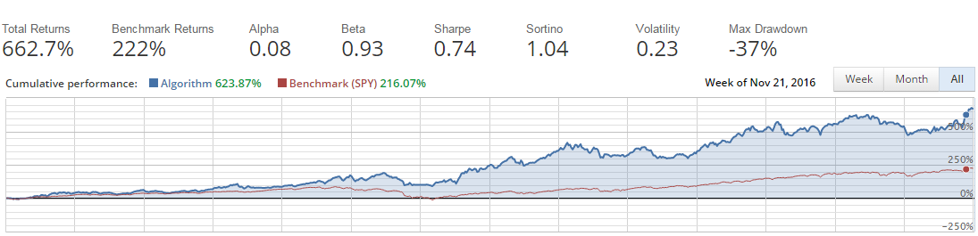
Simple Equity Momentum
You want more details. Fine, more details coming below. Oh, and the report below is totally automated in Quantopian.
I hope this little example could help you get started and play around with Python. Quantopian is a good place to start. See it as the gateway drug. Play with this code first and get the hang of the basics. We’ll get back to syntax and structure of the language another time.
SimAnalysis


Awesome stuff! You got me started in Quantopian and Python with this article. I want to build a solid equity strategy to run together with my trend following system on futures/CFDs. One question. What development environment (IDE) do you use to develop your code? Visual Studio, Spyder, Pycharm..?
I’m trying out Visual Studio for now.. The Quantopian web-based scripting in the site has very limited auto-complete and error checking functionality.
Thanks, Carlos. I’m working in multiple environments at the moment, but mostly Spyder. Most I’ve spoken to who have been doing this much longer than I have tell me that they use either VS or Jupyter Notebook.
To be honest, I found the Quantopian web environment annoying to start off with, but I’m really starting to like it.
astonishing! incredible stuff Andreas. Thanks for sharing!!!
Thanks for sharing the code and text, Andreas!
As for IDE, I have good experience with PyCharm (www.jetbrains.com/pycharm) and SublimeText (www.sublimetext.com).
In general, Java and C# developers use IDEs, that usually integrate pretty much everything, but its basically GUI covering-up collection of tools in background – style/type-checker, compiler, etc. But you can run those on your own for your greater flexibility via Terminal (or Vim/Emacs/Sublime plugins). Once learned you can leverage it in so many other areas!
Thanks for posting this, Andreas. Great into to the magic of python and Quantopian. Have a great 2020 and beyond.